Xpírijensis astrofotografa

You think it’s a rare case? Nope! In summer 2012 I got a new Atik 460 EXM with really misaligned CCD chip. How I did I find that? I have some really perfectly collimated optics (setups) so unlike of 99% of other astro-imagers who face all kind of issues and never can exactly tell which piece is on blame in their imaging train I can easily test such a case. On top of that, I have this kind of experience from 2010 when I beta tested first KAI-11000 based CCD camera for Moravian Instruments.

Because people tend to skip reading whole story (important details) I will make a conclusion right away. Moravian Instruments shall deliver all their CCD cameras with properly aligned CCD chip since summer 2010 when I insisted on this as a must-have and fundamental thing. In late 2012 I got a replacement Atik camera which had the chip finally well aligned (it was kind of a luck). Since I like Atik and am a big fan of their SONY based cameras (I recommend them, especially ICX694 ones over popular KAF-8300 based) I shared my experience with the CEO of Atik (Steve). Here’s what he responded: “you will be pleased to hear that we are working on a new mounting system that should provide a better performance in this respect ”.

Now, let’s see some images of a properly working system, misaligned system using the same setup and some demo-images to show how a wrong and correct image (star field) looks like with regards to chip alignment issue mentioned in this article.

Carl Zeiss Lens @ F/2.8 using APS size chip of QHY10

Carl Zeiss Lens @ F/2.8 using 16mm diagonal of Atik460EXM

The star image looked focused on the left side and defocused on the right side. That was my concern. Since I replaced the camera with other Atik 460 EXM, I am much more happy as the new one is OK

To demonstrate how the star image with misaligned sensor (or other tilt in your imaging system) might look like I decided to use the two from 2010 because the Lens-example above with QHY10 and Atik460 doesn’t look so horrible (obvious) due to expected distorsion from wide open lens (F/2.8).

Misaligned case (tilt in the system)

Aligned case (no tilt at all)

To chase the tilt in your imaging system (CCD camera, filter wheel, rotator, threaded connections etc.) using flat field analysis can help.

Flat - Atik460 - Misaligned case

Flat - MII G3-11000 - Aligned case

At the moment (late 2013) I own two mono CCD cameras both with well aligned CCD chip and both performing perfectly (Atik460EXM for narrow band imaging and G3-11000 for LRGB imaging).

OK, it won’t be actually the first light, but a brief report from a third night (third use case) when I finally managed to handle the setup (cables etc.) and master polar alignment of this new friction drive mount made by Gemini Telescope Design in Hungary.

On the first night I messed up polar alignment because I did not purchase the polar scope (I was too cheap and did not want to spend any more money on additional astro equipment). I was hoping that I can do the PA with a method I learned from my astro-buddy (Pavel Vabrousek) that we were using in Chile in 2010. It’s based on simple comparison of two rather widefield images taken with a CCD camera of a rotating sky around the pole when the mount is completely stopped and when the PA axis of the mount is manually rotated during the other image capture. This way you get two images where you locate the point (X-Y position) of the spot that is the center of the circles and the goal is to match them to overlay using ALT/AZ screws of the mount. This sounds simple (and is very precise), but as there were freezing -11 degrees out there I did not have the mood to mess with it for longer than 30 minutes. Therefore my PA was too off (after PA I bumped into the mount when loading counterweight) to say anything about the mount performance. And before I started taking images, the clouds rolled back in. The 3 hours lasting clear sky window we had on 11th of February 2013 ended and I drove back home 100 km without any photons collected. More over that – I was then sick for next few days because of the cold weather – I spent another hour with attempts on GoTo alignment that first night.

On the other (second) night I already had the polar scope, but I did not collimate it well in the first instance and I did not read the proper instructions how to use it (not mentioning I should know it all as it’s very similar to my previous mount) which resulted in, again, poor PA. So at least I took some binned image as a first image of year 2013 (during first 5 moths of this year we had 5 nights of some (3 – 5 hours lasting) clear sky – it’s a total pain so I was happy for at least something to play with).

On the third night, I finally did everything just fine and was stunned by the tracking performance and quality of the mount. OK, there are few minor details about the mount, but I am too big nitpicker who is able to find critics (even subtle, but reasonable) on everything I had in my hands ever. Want to hear the conclusion? The unguided 6 min subs I took that night (for a certain reason I went with only 6 min subs that night) were totally equal to guided 6 min subs. But I was using short focal length setup with too big image scale (2.83 arc-seconds per pixel). Let’s see some images now. First image shows my nice setup

Third use case of Gemini G53F in the field.

And second image shows the tracking error graph as smooth as I have never seen it before.

Tracking Error Graph of Gemini G53F

Even though I did not measure PE yet (I even do not plan to do so as I know it’s very small with zero backlash) I think it’s obvious how good the mount tracks. Since I was using many previous mounts with the exactly same setup (guiding with miniBorg 50 using MII G1-0300 CCD camera) I think it’s “fair” to compare the tracking error graph from Losmandy G-11 Gemini and Sky-Watcher HEQ-5 mounts as can be seen on third and fourth image below.

Tracking Error Graph of Losmandy G-11 GoTo

Tracking Error Graph of SkyWatcher HEQ-5

I really liked my first real astro-mount the SW HEQ-5, I even still own it as it’s nice, lightweight and convenient for a short refractor imaging. I was really impressed by the quality of my other mount I had, the Losmandy G-11 Gemini GoTo, but as my imaging skills improved I became more and more demanding on the imaging equipment. The Losmandy was perfect until I used a 2800 mm focal length telescope with an Off Axis Guider. Also, as I like to stay on the safe side (in all circumstances) I tend to use overkill setups. And I knew that one day I will “have to” use a Newtonian telescope because it simply collects much more light then any affordable refractor and would have zero chromatic aberration, which is something I have not experienced before. Because couple of my friends were happily using Gemini G42+, the predecessor of G53F (F stands for friction drive mount) for even unguided imaging, it was a clear choice which mount will be my final one The choice was sooo easy because you get top-notch performance for half of the costs of e.g. Astro-Physics mounts or Paramount (range starting at 9.900,- eurodollars). In the similar range there’s also Mesu 200 mount, but that caught my eye only as a top candidate for ugliest design ever seen (and I care about design, I love things that work and that look good). Advertised 4” peak to peak PE seems to much to me as I hope for half of that with G53F and you know what, advertised not always equals reality (reality is worse then what we hope for). On first look the 65kg or 100kg loading capacity is a total non-sense just from a brief look on the mount head that is no more rigid than “poor” G53F aimed at 45kg of load. That’s enough of critics of something I never had in my hands so please, dear readers, do not take my words seriously, I am an extraordinary guy with shifted mind! So far, all mounts I have purchased were good decision so I believe (I hope ) this third one would be too.

Anyway, there are couple of things that I do not like. Mainly it’s the Pulsar 2 controller that I find way too user unfriendly. It’s different than what I was used for from Losmandy’s nice GoTo handpad. But I have already learned how to use it and the major drawback (missing catalogs for GoTo) is resolved now (see LBN, LDN, Sh, and stars by Pavel P.) though you still have to (at the time of this writing) upload them into e.g. Planets (e.g. LDN counting almost 2000 of objects) or User (has 500 entries) for Sh-2 catalog having 313 objects, or other sections as these base names are fixed. Another thing is driver for MaxIm DL (or ASCOM) that doesn’t work 100% well, I am having some issues with it, but found a way how to use the mount (guiding over telescope connection) so it’s fine. From mechanical point of view I was more happy with setting up Losmandy G-11 that was lot more easier to do – also having elevation scale and two axis bubble level was a nice feature of Losmandy (the G53F is fixed by one screw from the tripod pier while the G-11 had three side screws and was easy to put on the tripod – with G53F I have to be more careful when putting it on the tripod pier). Polar scope of Losmandy G-11 was much easier to use, but on the other side – the G53F is completely different performance level equipped with off-axis polar scope and the best news about the HP-2 polar scope is – that it holds the collimation well so you do not have to bug with it every single time if you store it carefully). The HP-2 polar scope has bigger aperture and magnification and therefore the PA is more precise then with Losmandy. And that really counts. With G53F you jump into a mature world of professional equipment where the details you never cared about (refraction correction, mount modeling parameters, balancing etc.) get their meaning. What I really like on G53F apart from performance/costs ratio and the fact it looks cool enough is that the current hand controller (I like to use HC I am used to it) has integrated GPS receiver so I do not have to bug with coordinates setup every single time I go out for imaging (I am mobile photographer having to setup every time from scratch).

Let’s end with a first light image result:

QE is the ability of a detector to turn incoming photons into useful output. It’s computed as detected photons divided by incoming photons. In other words, a CCD sensor/detector with say 70% of QE detects 7 out of 10 incoming photons. That’s what simplified theory says. For an astronomical CCD camera that aims to detect dim objects within some kind of light spectrum it is one of the key parameters. It’s a parameter of major interest, but it is not the only one that matters (because low QE camera can still bring good results in some applications as far as the chip size is huge and we have good enough optics that allows to use large, full size chips). The other key parameter (to make up a pair of what is fundamentally important) is the noise (particularly readout noise as the other sources could be dealt with, at least in some extent). Noise (readout noise) is a chip property. It can vary by a hair (or two) in the same chip lineup (e.g. within the same family – chip name). Moreover the chip readout noise differs among various camera makers using the same chip name (family) in their cameras (as a CCD camera is very sensitive electronic device that requires good electronic design and high quality parts to be used). To this research I devoted following article: CCD Camera Noise Tests and Comparison

Therefore an IDEAL astronomical CCD camera would have:

Recently, I have seen a very nice QE comparison chart made by Philippe Bernhard that I must share with you (re-publish) as it’s really nicely done and shows today’s most popular chips’ QE curves of KODAK KAF-3200, KAF-1603ME, KAI-11002ME, KAF-8300ME, KAF6303E, KAI-4022, KAF-16803 and SONY ICX285, ICX674 / ICX694.

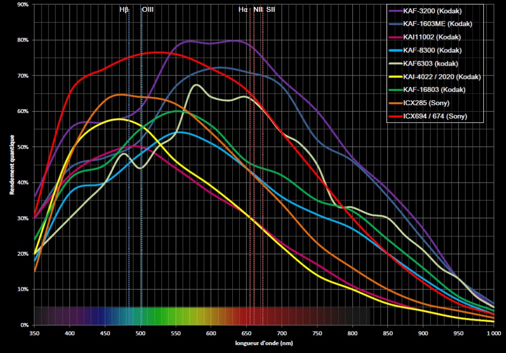
Most popular CCD's QE Comparison Chart made by Philippe Bernhard

What’s remarkable is the “difference” between Kodak KAF-3200 (costs a fortune – too pricy sensor with huge(!) noise levels and on top of it being NABG which means it’s not the best choice for an astronomical photographer who wants to make pretty pictures without care of blooming) and Sony ICX694 (or ICX674 that’s the same chip, but of a smaller size) that has really low noise. The size of chips is similar, but Sony ICX694 / 674 is half the price of KAF-3200 and delivers very clean images (I am not afraid to say that you get two to four times better camera for half of the price). It will just shine in narrow band imaging. Another remarkable fact is the difference between today’s very popular Kodak KAF-8300(ME – all are micro lens enhanced chips) and Sony ICX694 / 674. Based that KAF-8300 has e.g. in H-alpha the sensitivity of 44% and ICX694 has around 68% there’s a difference of a factor 1.5 times in favor of Sony. On the other side, the KAF-8300 is bigger (not so bigger in width/height dimensions, but twice bigger in surface size), but again, on the other side, ICX694 has far less noise and delivers much cleaner images so it’s question whether FOV matters to you or not (FOV can be adjusted by using shorter focal length telescopes or more powerful focal reducers on the same aperture telescope). Last remark to point out is the QE of KAI-11002ME. Looks horrible (and it is horrible, in namely H-alpha shooting – from my experience it’s disaster), but in LRGB it is usable and considering the really big size of the chip it can still deliver pretty nice images when matched to an expensive astrograph that is tracked on an expensive mount. Downside of cameras with this chip is the weight and additional stress on focuser (requiring a few grands more expensive focuser).

There are many QE charts available on the Internet so I show only one more made by Point Grey Research, Inc. that covers comparison of QE of following chips: SONY ICX674 / ICX694 (both EXview HAD II), IMX035, CMOSIS CMV4000, SONY ICX445, ICX285, ICX625 (both EXview HAD) and Aptina MT9V022 CMOS.

CCD's QE Comparison Chart, (c) Point Grey Research, Inc.

Notice the difference (subtle) in Sony ICX285 (grey) and Sony ICX445 (yellow) in favor of ICX445. It’s really interesting how a chip with smaller pixel size (3.75um of ICX445 vs. 6.45um of ICX285) can be equal or even better in terms of QE in comparison to highly acclaimed Sony ICX285. The answer to this mystery is the new SONY technology named EXview HAD II. Sony ICX445, ICX674, ICX694 are all new generation CCD chips with EXview HAD II technology. See image and link below. But to be completely honest with you, reader of my mental brainstorm, the smaller pixel cameras do really have a bit higher readout noise (which is what we do not want), but surprisingly the higher QE compensates for it! I will devote another upcoming article to this problematics and closer comparison of Kodak KAF-8300 vs. Sony ICX694/ICX674 chips later.

Sony Exview HAD vs. new Exview HAD II

For more information check http://www.sony.net/Products/SC-HP/cx_news/vol62/np_icx674alg_aqg.html and http://www.sony.net/Products/SC-HP/cx_news/vol52/pdf/featuring52.pdf

Also notice how good is the new Exmor CMOS based chips (family IMX). This one is found in planetary cameras these days as well as popular ICX618 that is superior than ICX445, but only by little! ICX618 is 1/4” (way too small with only 0.3 megapixels) and ICX445 is 1/3” (small) with decent 1.2 megapixels. My future, soon to be released, guide and planetary and meteor trails capture camera will feature ICX445 (new MII G1-1200 from Moravian Instruments) SEE UPDATE at the bottom of this article! Again, the ICX674 (green) is equal to ICX694 (ICX694 is 16mm diagonal while ICX674 is 11mm diagonal both have same pixel size). The newest EXview HAD II Sony based astronomical CCD cameras can open new doors and bring us to new horizons (or even beyond ). I would say it’s a revolution in amateur astronomical imaging. I have it all except of clear skies.

Conclusion? Best is to have more then one CCD camera, each selected according to intended use - for shooting small objects like tiny galaxies or planetary nebulae you may get small chip sized camera but powerful one (high QE, low noise) while for large wide field imaging you may get as big chip as possible (like 36x24mm) that allows to capture large amount of sky without wasting time and effort on doing mosaics. Other benefit is that it allows to use big aperture telescope to collect more photons. Big aperture telescopes usually have longer focal length and slower F-stop ratio, but you can HW bin 2×2 in order to make the system faster (from say F/10 using bin 1×1 you can actually go down to F/5 with bin 2×2 – therefore big chip can serve you as a focal reducer (as long as the optics can support it – has flat field) and many megapixels guarantee you still end up with decent pixel dimension of the image). Does it match your wallet?

This Article is a follow up on a post I wrote earlier for a czech astro magazine: Současné CCD kamery pro fotografování DSO, stručný přehled.

More QE charts for ICX445 compared to its alternatives could be found here: http://www.ptgrey.com/support/downloads/documents/TAN2008006_Sensor_Response_Curve_Comparison_for_ICX445.pdf

UPDATE
Theory and praxis. Two different worlds. In praxis, it looks that ICX445 is JUST A BIG DISAPPOINTMENT.

Really? Really. Since 2008 when I purchased my first (ever) refracting telescope intended for astrophotography (Borg 77 EDII @ F/4.3) I have collected many Borg items purchased from Astro Hutech (Ted Ishikawa was always very helpful). Namely, after Borg 77 EDII with F4 Super Reducer (#7704) I got Borg 45 EDII with #7866 triplet reducer. Then I got Borg 71 FL with new #7870 triplet multi super reducer, #7887 0.85x DGL reducer and #7878 yet another triplet super reducers to be used for narrow band imaging with a 3rd party achromatic telescope and various CCD cameras. Last (but not least) lens was Borg 50 to be used as a guider (perfect lightweight and compact). It’s said that one image is worth a thousand words so here we go (it’s just a part of my collection that I was able to locate):

Borg Parts

Some Parts

New Mini 71FL

Borg scopes are very good performers (taking into account how fast they are) and perfectly lightweight. The weakest link in the imaging train, from an astrophotographer’s perspective, are all of the helical focusers. For AP be sure to get FTF instead!

Borgs in Action

References
AstroHutech – BORG
Joining the Borg – S&T Review by Alan Dyer
Borg 77EDII Astrograph – an user “review”

OK, it’s not going to be a real review, but just a bunch of user comments after using this camera for a while. First, I’d like to state the reasons why did I purchase it? I wanted a camera that is color (OSC, one shot color) because I own only couple of mono cameras. I wanted to experience ADC settings on my own and test its impact on real noise characteristics (readout noise etc.). I wanted the color version for constellation photography and for comet imaging (do rarely, but some day it could be handy). In time-limited imaging sessions (like on a vacation – once per year) it’s good to collect the same amount of data over all three color filters (Red, Green and Blue). With mono I have many times ended missing one of the three channels (because for best results you always have to refocus between filters no matter how parfocal they are so you can’t shoot R/G/B/R/G/B sequence). So my vision was to use the camera once per year (or few times) on a vacation to shoot color images in places with as low light pollution as possible (it turned out to be hard to find these skies on a family vacation, therefore next time I plan shooting narrow band only) on say Astrotrac platform (that only allows for 2 hours of tracking without rewind and reworking the composition of the image – with AZ head it’s easy to re-composite, you only have to rewind the RA (azimuth) axis). The initial vision was to use a field-power box (LiPO battery pack) with limited capacity in order to be low-weight due to portability reasons.

This is strictly a person subjective sum of points from a most demanding astro-imager on the planet Earth. Your experience will most probably differ to mine.

Here are the weak points:

two-frame readout mode (no progressive scan readout) which is maybe even worse than interlined readout (which in fact, without mechanical shutter makes things even more complicated – but on the other side what’s missing can’t get broken ). The problem is that you really need to take good set of bias frame in order to calibrate e.g. flat field calibration frames to remove the color gradient that appears in the image if you do not calibrate well your raw light data.

 
Here are some strong points:

 
Why did I sell it? [new was for 2.400 EUR, sold my tested and proven for 1.520 EUR!]. It did not meet my expectation and the reasons why I purchased it. Now I have switched to Sony ICX694 (new generation ExView HAD II) chip-equipped mono CCD camera. I prefer high sensitivity and low noise with much smaller FOV (but insanely nice narrow band capabilities) than large (and color), but dim picture to complement my large format camera. For large FOV I will keep my MII G3-11000 CCD (mono, of course) because that’s the best (and cheapest) camera with the damn noisy KAI-11002ME CCD for an European citizen at the moment.

Related QHY articles:
Set-Point TEC Cooling Tests of QHY CCD camera
QHY10 – Binning, Gain, Offset, Noise, Light Response etc.

To complete my complaints monolog, I should show some of my images done with this CCD camera:
Pavel Pech, QHY10 OSC CCD

QHY10 two frame readout mode

QHY10 single and master bias frame

Seeing is believing. I like to check and measure myself various characteristics and parameters of new items that I have just purchased. The purpose is to show how good or bad the product is in order to make it easier for other astrophotographers (I usually buy only photography stuff) to make the purchase decision. This time, I got another chance to use the Carl Zeiss Jena SPECORD M400 spectrophotometer so I took the filters I haven’t measured yet and did a full spectrum run.

First, let’s see IDAS LPS-P2, the highly recommended and popular filter (almost a must have for one-shot-color cameras) to fight against light pollution. Personally, I call this filter a “soft-LPS” (or soft-CLS) and I use it at locations with only slight light pollution (e.g. in a National Park or simply at the best dark sky locations I usually shoot at). LP is unfortunately everywhere (in my case). The best on this filter is that it allows for good color calibration. It doesn’t eat that much of yellow-red colors like a typical CLS filter does (see below). The downside is that it works best in dark sky locations and is not very strong in the fight against light pollution.

IDAS LPS-P2 spectrum plot

The measured chart (above) of an IDAS LPS-P2 perfectly matches manufacturer’s chart so it really delivers what it advertises (as in fact all of these filters, this time).

Next, let’s see IDAS LPS-V4. Personally, I call this filter “OSC-narrowband” as it blocks everything except of a “narrower” bandpass around OIII (500nm) and around Hydrogen Alpha (656nm) so it is useful to capture this kind of signal in one shot which, in case of an OSC camera, makes use of all RGGB Bayer color planes (unlike of e.g. pure H-a filter that when used with OSC CCD renders green and blue color planes useless – as they contain only noise).

IDAS LPS-V4 spectrum plot

The only thing I do not like on this filter (I am very demanding customer) is that there’s a bit of leak (topping 25% of transmittance at around 377nm) in UV part of the spectrum – this is not very good for cases when you use poorly corrected optics in UV (almost every objective lens – refracting optics – has this kind of “issue”). On the other hand, it matches manufacturer’s plot so there’s no intention to hide this subtle imperfection. If I am a filter manufacturer I’d make a filter similar to this one but with no UV leak and with even much narrower pass at the OIII and Ha emission lines (Ha with NII and maybe also with SII lines) that would serve very well for “narrowband Luminance channel” Just my sci-fi vision (I’ve got plenty of such stupid ideas).

Next is Astrodon Sloan z’ filter that I purchased for some experiments in infrared shooting (I use it as IR-Luminance – actually I have used it only once). This filter should block visible light and pass signal starting from 820nm of wavelength. My test proves it is really a digital filter passing 0.07% of visible light and around 821nm it takes off (with 7.1% of transmittance) over 55.5% of transmittance at 827nm and 98.6% at 833nm. There is no leak anywhere in 200-900nm.

Astrodon Sloan z spectrum plot

Last filter I tested was Baader UV/IR Block (should block everything but 420-680nm), #2459210A. This one also performs very well and it is one of two Baader filters I like very much (I do not like the rest though (for many reasons) – not talking about Astronomik filters that I do not like all of them (again, for many reasons)). This filter has really great transmittance of 97% to 99% and is currently the only UV/IR solution for refractors where we do really want to cut the UV part (below 400nm) as many refracting optics is poorly corrected in blue. It gets even worse with top-notch / perfect-most filters on the planet Earth – Astrodon filters – in conjunction with a very sensitive CCD camera, where the Blue filter takes off quite early in UV part and has very high transmittance (97-99%) right away – this is very OK and perfect for reflecting optics, but not for refractors – maybe should Astrodon offer two kinds (sets) of Blue filters (the Blue ones are in fact equal for both E-series (Sony ICX, Kodak KAF detectors) and I-series (Kodak KAI detectors) – I do own both sets).

Baader UV/IR Block spectrum plot

That’s it .